2回目ワクチン接種完了
ようやく2回目のワクチン接種完了
そんなわけないけど、なんか高揚感があるような感じで何かを感じる(気分の問題。)
抗体価の上昇をなんとなく感じる(そんなわけないか)
— くろたんく@激しく多忙 (@black_tank_top) 2021年9月15日
明日は具合悪くなるだろうけど、横になりながら本くらい読めたり、NETFLIXとか見られるくらいの元気だけは欲しいな。
今日から10-14日くらい経てばFully Vaccinatedってことで例のアイコンをつけたい。
SELFIES, a new molecular representation method
I was thinking of writing my own explanation of SELFIES, partly because I couldn't find a detailed Japanese explanation of its grammar anywhere, and partly because I wanted to use it for my own research and wanted to deepen my understanding. Then, Mario Krenn, the first author, contacted me and said I could write about SELFIES on my blog. From there, I reread the paper a bit, examined the differences in behavior between the current version of SELFIES and this version, and came to an almost complete understanding of the grammar, which I wrote about SELFIES in Japanese in my blog.
And also I participated in the SELFIES Workshop on August 13, 2021.
accelerationconsortium.substack.com
Some of the participants asked me if there was an English version equivalent to the Japanese explanation I wrote. So I have translated it back into English.
Introduction
This article is an introduction to SELFIES, a new molecular representation presented in this paper, developed in the lab of Prof. It was developed in Prof. Aspuru-Guzik's lab, who is famous for creating Chemical VAEs. (It will be up on arXiv in 2019)
Original title: Self-referencing embedded strings (SELFIES): A 100% robust molecular string representation
Authors: Mario Krenn, Florian Häse, AkshatKumar Nigam, Pascal Friederich, Alan Aspuru-Guzik
Journal: Machine Learning: Science and Technology
Publish: 28 October 2020
doi: 10.1088/2632-2153/aba947
I have written this paper for brevity and clarity, based not only on the paper, but also on my understanding of the behavior I have seen in running the code and the implementation, so please refer to the paper and the implementation if you are interested.
If you are interested, please refer to the papers and implementations. Also, the contents of this article are based on the latest version, v1.0.4.
[Note] Since the development has been going on since the paper was published, there are some discrepancies between the description in the paper and the output in v1.0.4. (I got stuck there...).
Outline of the paper
SMILES is widely used as a standard string molecular representation for chemical compounds, but when SMILES is used for input and output of generative models, there is a problem that a large part of the molecules do not correspond to valid molecules. The reason for this is that the generated strings are syntactically invalid or violate basic chemical rules such as the maximum number of valence bonds between atoms. The authors seem to have developed SELFIES to solve these problems.
Even a completely random string of SELFIES can represent a correct molecular graph. To achieve this, the authors developed SELFIES using ideas from theoretical computer science, namely formal grammar and formal automatons (formal Chomsky type-2 grammar (or analogously, a finite state automata)). In the paper, describe the development of SELFIES.
In the paper, we tried VAE and GAN with SELFIES and SMILES, and the results show that the output is fully valid and the model can generate orders of magnitude more molecules with SELFIES than with SMILES. (Table 1, Figure 5, Figure 6)
The great thing about SELFIES (in my opinion)
Instead of using strings to indicate the beginning and end of Rings and Branches, SELFIES represents Rings and Branches by their length, and avoids syntactic problems by interpreting the symbols following the Ring and Branch symbols as numbers representing their length (Index Symbols, to be discussed later).
Coding considering bond valence. It is designed to ensure that the physical constraint that C=C=C is possible (three carbons connected by a double bond), but F=O=F is impossible (F can only have one bond and O can only have two bonds) is met.
I have tried VAEs of Mol to SELFIES and Mol to SMILES using graph neural networks myself, and the generation of both SMILES and SELFIES works well, but most of the SMILES are not valid (several percent), while 100% of the SELFIES are valid. However, with SMILES, most of them are not valid (a few percent), but with SELFIES, they are 100% valid. (The details of the results of the test will be discussed another time.
Other results using SELFIES
Based on the results in the above paper, I believe that SELFIES will perform well in the task of inverse design of functional molecules based on deep generative models and genetic algorithms. We have already obtained a number of results using SELFIES.
- Inverse design using genetic algorithms
- Conversion from molecular images to SMILES
- Conversion from SMILES to IUPAC-name
The grammar of SELFIES (main topic)
About SMILES
If you don't know anything about SMILES, this article won't make any sense at all, but I'm going to assume that you do know something about SMILES.
If you don't know what SMILES is, I suggest you read py4chemoinformatics first to build up your domain knowledge, including how to use RDKit.
It's English version repository (original repository is here)
MDMA Explained (just look at it for now)
Now, let's start the explanation.
First of all, the SMILES of MDMA (3,4-Methylenedioxymethamphetamine), which appears in Figure 1 of the paper, is written as it is. MolFromSmiles("CNC(C)CC1=CC=CC=C2C(=C1)OCO2") in RDKit, it will be drawn as follows.

So, the SMILES of MDMA is CNC(C)CC1=CC=C2C(=C1)OCO2.
On the other hand, what happens to the SELFIES of MDMA?
import selfies as sf
sf.encoder("CNC(C)CC1=CC=C2C(=C1)OCO2")

# [C][N][C][Branch1_1][C][C][C][C][=C][C][=C][C][Branch1_2][Ring2][=C][Ring1][Branch1_2][O][C][O][Ring1][Branch1_2]
At this point, let's close the paper, because it's not the same as the expression of SELFIES in the paper (I know that the result is the same (it's just that this is how it was expressed in the version at the time)).
If you read Figure 2 properly, you may be able to understand it, but at first glance it doesn't make sense. First of all, the number of "C" seems to have increased compared to the original SMILES. It's hard to understand with MDMA, so I'll use a simpler example.
In order to understand the grammar of SELFIES, you need to understand Atomic Symbols, Index Symbols, Branch Symbols, and Ring Symbols. If you can understand these, you should have no problem.
Atomic Symbols
Let's start with an appropriate example.
sf.encoder("C=CC#C[13C]")
# [C][=C][C][#C][13Cexpl]

sf.encoder("CF")
# [C][F]

sf.encoder("COC=O")
# [C][O][C][=O]
Atomic Symbols are composed of a bond type, which represents the bond type, and an atom type, which is represented by SMILES and denoted by .
The bond type is the same as in SMILES.
- single bond : '' (empty)
- double bond : '='
- Triple bond type: '#'
- Geometric isomerism: '/' and '\\'.
Atom type is the same as SMILES. However, if you explicitly use brackets (), such as [13C] or [C@@H], the character expl is added. Ions are also possible.
One of the reasons for the high Validity of SELFIES is the Decoder. Let's look at an example.
sf.encoder("COC=O")
# [C][O][C][=O]

sf.decoder("[C][O][C][=O]")
# COC=O

# Even if you ignore bond valence and write an appropriate compound, it will only be decoded to the part that is possible.
sf.decoder("[C][O][=C][#O][C][F]")
# COC=O
If the bond constraints of the previous or current atom are violated in this way, the bond multiplicity is designed to be reduced (minimally) so that all bond constraints are satisfied. (There is a description that gives the valence here: XXXXX_bond_constraints)
So far, I think you can understand the case of a simple linear chain. Next, I will explain the Branch Symbols and Ring Symbols, but before that, I would like to explain the Index Symbols, which are necessary for the explanation of Branch Symbols and Ring Symbols. This is because the Index Symbols, which are essential for the explanation of Branch Symbols and Ring Symbols, need to be explained first.
Index Symbols
This is where I personally got very stuck (and didn't notice it), but as I mentioned above, here are the key points.
- The beginning and end of a ring and branch in strings, SELFIES represents rings and branches by their length.
- After a ring and branch symbol, the subsequent symbol is interpreted as a number that stands for a length.
What this means is that you can think of index as a string that represents an atom, branching structure, or ring structure.
You can find the description here.
The table below shows the results.
| Index | Symbols |
|---|---|
| 0 | [C] |
| 1 | [Ring1] |
| 2 | [Ring2] |
| 3 | [Branch1_1] |
| 4 | [Branch1_2] |
| 5 | [Branch1_3] |
| 6 | [Branch2_1] |
| 7 | [Branch2_2] |
| 8 | [Branch2_3] |
| 9 | [O] |
| 10 | [N] |
| 11 | [=N] |
| 12 | [=C] |
| 13 | [#C] |
| 14 | [S] |
| 15 | [P] |
The symbol 𝑄 is used a lot in the paper, and this is what it means. Thinking in terms of hexadecimal numbers, 𝑄 can be expressed as 𝑄 = (idx(𝑠1)×162)+(idx(𝑠2)×16)+idx(𝑠3).
To see what I mean, let's take a look at the Branch Symbols example.
Branch Symbols
Now that we can use Index Symbols to calculate 𝑄, let's look at an example with a branch structure.
# SO4
sf.encoder("S(=O)(=O)([O-])[O-]")
# [S][Branch1_2][C][=O][Branch1_2][C][=O][Branch1_1][C][O-expl][O-expl]
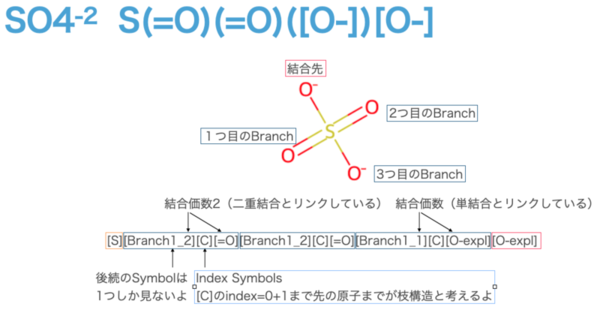
First, Branch Symbols has the pattern [Branch{L}_{M}]. The L on the left is the range {1, 2, 3}, and the number means how many subsequent letters are to be seen as Index Symbols. 1 means one letter, 2 means two letters, and so on. In this example, we are not looking at the second letter, so we need to assume that the second letter is a long chain, for example, "C" is more than 17 characters long (more on this later).
Next, the M on the right side of [Branch{L}_{M}] is the range {1, 2, 3}. This shows the bonding pattern with the atoms after the Index Symbols. 1 for a single bond, 2 for a double bond, 3 for a triple bond, and so on. Of course, the target Atom Symbols are linked to each other. By the way, if either one of them is not satisfied, the lesser one will be preferred, because the bond multiplicity is designed to be reduced (minimally) so that all bond constraints are satisfied if the bond constraints of the previous or current atom are violated.
If we consider the case of [Branch1_2] using SO4 as an example, only [C] will be processed as an Index Symbol, since subsequent Index Symbols will only see one character. In the table shown above, [C] has an index of 0. It is important to note that the branching structure is calculated from the Index Symbols, 𝑄, and is considered as a branching structure up to 𝑄+1 th symbol. In this case, all of them are [C], so the branch structure is up to the first letter after that ([=O] or [O-expl]). It is easy to understand that Atomic Symbols, without Branch Symbols, are directly connected to each other. (In this example, the head and tail are directly connected, and the other three are branch structures (orange and pink symbols).
(In this example, the head and tail are directly connected, and the other three are branching structures. (Up to Branch 3 is possible, so something as long as 16 ** 3 is possible.
Ring Symbols
Now that you understand it, Ring Symbols is very easy.
There are two main patterns of Ring Symbols: [Ring] and [ExplRing], where L is {1, 2, 3} and the number of subsequent letters are considered as Index Symbols or not. Then, it calculates 𝑄 in the same way as Branch Symbols, and combines it with the 𝑄+1 th previous Atomic Symbols to form a ring structure.
Well, let's look at an example. Everyone's favorite :) Benzene rings are easy to understand.
sf.encoder("C1=CC=CC=C1")
# [C][=C][C][=C][C][=C][Ring1][Branch1_2]
#  ↑   ↑  ↑   ↑  ↑   ↑
#  5   4  3   2  1   0
It is important to note that after [Ring1] are Index Symbols. You see [Branch1_2], but this is just what we think of as an index. Since it is [Ring1], only one character after it is considered as Index Symbols. Since [Branch1_2] has 𝑄 = 4 in the Index Symbols table, the first Atomic Symbols is [C], which is the 𝑄+1st, In other words, the five previous Atomic Symbol is the first [C], which is joined to form a ring structure.
Also, [ExplRing] about this pattern is easier to understand if you think of it as another representation of a benzene ring. The benzene ring can be written as C=1C=CC=CC=1 in SMILES. If we use this as SELFIES, we get the following.
sf.encoder("C=1C=CC=CC=1")
# [C][C][=C][C][=C][C][Expl=Ring1][Branch1_2]
#  ↑   ↑  ↑  ↑   ↑  ↑
#  5   4  3  2   1  0
The basic idea is the same, but since [Expl=Ring1] is used, the bond type should be "=" when creating a ring structure with Atomic Symbols, which is the standard just before Ring Symbols. (You can imagine that =1 at the end of SMILES corresponds to [Expl=Ring1].
Extra for "Ring" use cases
Ring Symbols are a little more interesting, and triple bonds such as acetylene can be written with Ring Symbols. (In short, if you create a ring structure with a double bond in a part that already has a single bond, it will become a triple bond.
sf.decoder("[C][C][Expl=Ring1][C]")
# C#C
MDMA Description
If you can understand this far, you will have a complete understanding of MDMA as shown earlier.
import selfies as sf
sf.encoder("CNC(C)CC1=CC=C2C(=C1)OCO2")

# [C][N][C][Branch1_1][C][C][C][C][=C][C][=C][C][Branch1_2][Ring2][=C][Ring1][Branch1_2][O][C][O][Ring1][Branch1_2]

It's a little difficult to understand because I couldn't color-code it well, but if you use all the assumptions you've made so far, you can understand it without any problems.
The difficult part is around the middle, [Branch1_2][Ring2][=C][Ring1][Branch1_2], where the branch structure is connected by a ring structure, which is quite difficult to understand, but if you think about it a bit, you can understand it.
Colab
This time, I used Colab because I wanted to run it in my hand so that I could do some thinking and error. It is available for viewing, so you can probably modify it in your own way or download it and try it out.
Summary
I hope that you now have an almost complete understanding of the syntax of SELFIES.
So why do SELFIES written in this format work so well for generative models such as VAEs and GANs, unlike SMILES? I think it is very important that SELFIES represents 100% valid compounds even if they are randomly sorted, that it is super robust, and that as a result, there are no invalid regions in the latent space.
I am wondering if I can use it successfully in my own research.
References
SELFIES GitHub github.com
SELFIES extensive blog post aspuru.substack.com
SELFIES Official Document selfies.readthedocs.io
新しい化合物の分子表現法 SELFIESの日本語解説
20210817追記
公式レポジトリに、この記事のリンクが貼られました。
以前日本語で書いたSELFIESの紹介記事リンクが公式レポジトリに貼られた!!😎
— くろたんく@激しく多忙 (@black_tank_top) 2021年8月16日
I woke up in the morning and saw that the link to my Japanese article about SELFIES was added on the README of the official #SELFIES repository!https://t.co/l0fUzGATRb pic.twitter.com/5tNl3b9v8n
はじめに
本記事は、こちらの論文で発表された新たな分子表現であるSELFIESの紹介です。Chemical VAE を作ったことで有名な Aspuru-Guzik 教授のラボで開発されたものです。(arXivには2019年にupされています)
原題: Self-referencing embedded strings (SELFIES): A 100% robust molecular string representation
著者: Mario Krenn, Florian Häse, AkshatKumar Nigam, Pascal Friederich, Alan Aspuru-Guzik
論文誌: Machine Learning: Science and Technology
Publish: 28 October 2020
doi: 10.1088/2632-2153/aba947
論文だけでなく、コードを動かして見た動作や実装された内容から理解して、簡潔さ・伝わりやすさを重視して記述しているので、ご興味を持たれた方は論文や実装を参照してください。
また、今回は最新バージョンのv1.0.4における内容とします。
注意 論文発表後にも開発がかなり進んでいるので論文での記述とv1.0.4におけるアウトプットに若干の乖離があるため、本記事と内容が合ってなくて??となるかもしれません(というか私はそこでハマりました・・・。)
経緯
SELFIESの詳しい文法の日本語解説がどこにも見当たらなかったのと自分の研究に使いたかったので理解を深めたかったという理由もあり、自分で解説を書こうかなと思っていたら、First authorのMario Krennさんからコンタクトがあって、ブログでSELFIESについて書いていいという流れになりました。そこから少し論文を読み直し、現状のバージョンのSELFIESとの挙動の差を検討して、文法をほぼ完全に理解したので解説します。
論文概要
化合物を表す標準的な文字列分子表現として多く使われているのはSMILESですが、生成モデルの入出力にSMILES使うとかなりの部分が有効な分子に対応していないという問題があります。原因としては、生成された文字列が構文的に無効であったり、原子間の最大価結合数などの基本的な化学ルールに違反していたりします。このような問題を解決するために著者らはSELFIESを開発したようです。
全くランダムなSELFIESの文字列でも、正しい分子グラフを表現することができます。これを実現するために、著者らは理論計算機科学のアイデア、すなわちformal grammar とformal automatons(formal Chomsky type-2 grammar (or analogously, a finite state automata))を利用してSELFIESを開発しました。
論文上では、SELFIESとSMILESを用いてVAEやGANを試した結果,SMILESを用いた場合よりもSELFIESを用いた場合の方が,出力は完全に有効であり,モデルは桁違いに多様な分子を生成出来ることが示されています。(Table 1, Figure 5, Figure 6)
(個人的に思う)SELFIESのすごいところ
- SELFIESは、RingとBranchの始まりと終わりを文字列で示す代わりに、環と枝をその長さで表す。RingとBranchの記号の後に続く記号を長さを表す数字として解釈することで、構文上の問題を回避(後ほどでてくるIndex Symbolsのこと)
- 価数を考慮して符号化される。
- C=C=Cは可能(3つの炭素が二重結合でつながっている)だが、F=O=Fは不可能(Fは1つの結合、Oは2つの結合までしか不可能)という物理的制約を確実に満たす様に設計されている。
- 自分自身でもグラフニューラルネットワークを使って、Mol to SELFIES, Mol to SMILESのVAEを試しているがSMILESもSELFIESも生成自体はうまくいくが、SMILESだと殆どがValid(数%)にならないが、SELFIESだと100%Validになっている。(試した結果の詳細は別の機会に)
その他SELFIESを用いた成果
上記論文の結果から、SELFIESは深層生成モデルや遺伝的アルゴリズムに基づく機能性分子の逆設計タスクにおいて、優れた動作をもたらすと考えられます。すでに、SELFIESを用いて続々と成果が出ています。
・遺伝的アルゴリズムを用いた inverse design
・分子画像からSMILESへの変換
・SMILESからIUPAC-name への変換
SELFIESの文法の解説(本題)
SMILESについて
そもそもSMILESについてわかってないとこの記事自体、全然意味分かんないんだけど、SMILESについてはある程度わかっている前提で書きます。
SMILESってなんやねんっていう人はまずは、py4chemoinformaticsを読んで、RDKitの使い方も含めてドメイン知識を溜めるとよいかと思います。
また、金子先生の本を読んで化学データの解析とそれらを用いた機械学習を一通り学ぶのも良いかもしれません。

SMILESを含んだその他の分子表現について
こちらは、@steroidinlondonさんが簡単に説明していくれているのでこちらを一読されるとよいかと思います。
MDMA解説(とりあえず眺めるだけ)
さて、解説を始めていきます。
まず、論文のFigure 1にも出てくるMDMA(3,4-Methylenedioxymethamphetamine)のSMILESが書いてあるのでそれをそのまま、Colabを使って、RDKitでChem.MolFromSmiles("CNC(C)CC1=CC=C2C(=C1)OCO2")すると以下のように描画されます。
つまり、MDMAのSMILESはCNC(C)CC1=CC=C2C(=C1)OCO2ということですね。
一方で、MDMAのSELFIESはどうなるのでしょうか?
import selfies as sf
sf.encoder("CNC(C)CC1=CC=C2C(=C1)OCO2")

# [C][N][C][Branch1_1][C][C][C][C][=C][C][=C][C][Branch1_2][Ring2][=C][Ring1][Branch1_2][O][C][O][Ring1][Branch1_2]
この時点で、論文のSELFIESの表現のと違うので一旦、論文は閉じましょう(結果同じことだと言うのはわかります(当時のバージョンではこういう表現だったというだけ))。
ちゃんとFigure 2を読めばわかるのかもしれないが、とりあえずパっと見意味がわからない。まず"C"の数が元のSMILESより増えている様に見えます。いきなりMDMAで理解しようとするときついので、もっと簡単な例でいきます。
SELFIESの文法を理解するには、Atomic Symbols, Index Symbols, Branch Symbols, Ring Symbolsを理解する必要があります。ここがきちんとおさえられれば多分問題ないはずです。
Atomic Symbols
まずは適当な例を示します。
sf.encoder("C=CC#C[13C]")
# [C][=C][C][#C][13Cexpl]

sf.encoder("CF")
# [C][F]

sf.encoder("COC=O")
# [C][O][C][=O]
Atomic Symbolsは、結合種類を表すbond typeと、SMILESで表されるatom typeで構成されて[
bond typeはSMILESと同じで、
- 単結合なら ''(何もなし)
- 二重結合なら '='
- 三重結合なら '#'
- 幾何異性は '/', '\\'で
表現されます。
Atom typeはSMILESと同じです。ただ、[13C]とか[C@@H]みたいに明示的にカギカッコ([])した場合はexplという文字が付加されます。ちなみにイオンも可能です。
SELFIESのValidityが高いことの一つの理由はDecoderにあると考えています。例を見てみましょう。
# 上と同じものを再掲
sf.encoder("COC=O")
# [C][O][C][=O]

sf.decoder("[C][O][C][=O]")
# COC=O

# 価数を無視して適当な化合物を書いても可能な部分までしかデコードされない
sf.decoder("[C][O][=C][#O][C][F]")
# COC=O
この様に前の原子や現在の原子の結合制約に違反する場合は、すべての結合制約が満たされるように、結合多重度が(最小限に)減少するように設計されています。 (このあたりに価数を与えている記述があります。XXXXX_bond_constraints)
ここまでで、単純に直鎖の場合は理解できると思います。 次に、Branch SymbolsとRing Symbolsについて説明しようと思いますが、その前に先程のMDMAの説明中に"C"が増えてる様に見えると言う話がありますがそれは、Branch SymbolsとRing Symbolsの説明に必須のIndex Symbolsについて先に説明する必要があります。
Index Symbols
個人的にとてもハマったところ(気づけなかったところ)だったのですが、前述していますが以下がポイントです。
SELFIESは、RingとBranchの始まりと終わりを文字列で示す代わりに、環と枝をその長さで表す。
RingとBranchの記号の後に続く記号を長さを表す数字として解釈する。
これはどういうことかというと、原子、分岐構造、環状構造を表す文字列をindexと考えるということです。
このあたりに記述があります。
表で示すと以下の通りです。
| Index | Symbols |
|---|---|
| 0 | [C] |
| 1 | [Ring1] |
| 2 | [Ring2] |
| 3 | [Branch1_1] |
| 4 | [Branch1_2] |
| 5 | [Branch1_3] |
| 6 | [Branch2_1] |
| 7 | [Branch2_2] |
| 8 | [Branch2_3] |
| 9 | [O] |
| 10 | [N] |
| 11 | [=N] |
| 12 | [=C] |
| 13 | [#C] |
| 14 | [S] |
| 15 | [P] |
論文上で𝑄 という言葉が多用されますが、これはこのことです。 16進数で考えて、𝑄を 𝑄 = (idx(𝑠1)×162)+(idx(𝑠2)×16)+idx(𝑠3) という式にで表現します。
どういうことかというと例を見たほうが早いのでBranch Symbolsの例を見ましょう。
Branch Symbols
というわけで、Index Symbolsで𝑄の計算ができるようになったので、分岐構造がある例を見てみましょう。
# SO4
sf.encoder("S(=O)(=O)([O-])[O-]")
# [S][Branch1_2][C][=O][Branch1_2][C][=O][Branch1_1][C][O-expl][O-expl]
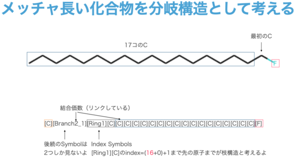
まず、Branch Symbolsは、[Branch{L}_{M}]のパターンがあります。左側のLは{1, 2, 3}が範囲で数字は、後続する何文字目までをIndex Symbolsとして見るかという意味です。1であれば1文字、2であれば2文字ですね。この例では2文字目まで見ているものはありません。2文字目まで見る場合というのは、たとえば"C"が17文字以上続くような、長い鎖を想定する必要があります(のちほほど紹介する)。
次に、[Branch{L}_{M}]の右側のMは{1, 2, 3}が範囲です。これは、Index Symbolsのあとの原子との結合パターンを示しています。単結合なら1, 二重結合なら2, 三重結合なら3といった具合です。もちろん、その対象のAtom Symbolはリンクしています。ちなみにどちらか一方を満たさない場合は、前の原子や現在の原子の結合制約に違反する場合は、すべての結合制約が満たされるように、結合多重度が(最小限に)減少するように設計されているので、少ないほうが優先されます。
SO4を例に[Branch1_2]の場合を場合を考えると、後続のIndex Symbolsは1文字しか見ないので、[C]だけがIndex Symbolsとして処理されます。ちなみに先程示した表で[C]はindexが0です。ここで注意したいのは、分岐構造がどこまで続くのかをIndex Symbolsから計算した𝑄で考えますが、𝑄+1 コのSymbolまで分枝構造として考えます。この場合すべて[C]なので後続の1文字目までが分岐構造です([=O] or [O-expl])
Branch Symbolsがなくなったものが、直結しているものと考えるとわかりやすいです。(今回の例だと頭とお尻が直結していて、その他3つが分岐構造のように考える)
ちなみに[Branch2_1]のようになるような例は以下の様なケースで、まぁ滅多なことでは登場しないでしょうが、このような長鎖であっても原理上は可能であるということです。(Branch3まで可能なので16 ** 3 というとても長いものが可能です)
Ring Symbols
さて、ここまで分かればRing Symbolsはとても簡単です。
Ring Symbolsは、大きく2つのパターンがあり、[Ring
まあ、例を見ましょう。みんな大好き(??)ベンゼン環がわかりやすいですね。
sf.encoder("C1=CC=CC=C1")
# [C][=C][C][=C][C][=C][Ring1][Branch1_2]
#  ↑   ↑  ↑   ↑  ↑   ↑
#  5   4  3   2  1  基準
ここで注意したいのは、[Ring1]のあとはIndex Symbolsです。[Branch1_2]と出ていますがこれはただのindexと考えるものです。[Ring1]なのでIndex Symbolsとして考えるのは後続の1文字だけです。[Branch1_2]はIndex Symbolsの表で見ると𝑄 = 4なので、𝑄+1番目前つまり5コ前のAtomic Symbolsは、一番最初の[C]ですね。これと結合して環構造を作ります。
また、[ExplC=1C=CC=CC=1と書くこともできます。こちらをSELFIESにすると以下のようになります。
sf.encoder("C=1C=CC=CC=1")
# [C][C][=C][C][=C][C][Expl=Ring1][Branch1_2]
#  ↑   ↑  ↑  ↑   ↑  ↑
#  5   4  3  2   1 基準
基本は同じですが、[Expl=Ring1]となっているので、Ring Symbolsの直前の基準のAtomic Symbolsと環構造を作るときにbond typeを"="にしてねっていう書き方です。(SMILESの最後の=1と[Expl=Ring1]が対応しているイメージで良いかと思います。)
おまけ
Ring Symbolsは少し面白くて、アセチレンのような3重結合をRing Symbolsで書くこともできます。(要するにすでに単結合がある部分に、二重結合で環構造つくると三重結合になるという仕組みっぽいです)
sf.decoder("[C][C][Expl=Ring1][C]")
# C#C
MDMA解説
ここまで来ると、先に示したMDMAが完全に理解できます。
import selfies as sf
sf.encoder("CNC(C)CC1=CC=C2C(=C1)OCO2")

# [C][N][C][Branch1_1][C][C][C][C][=C][C][=C][C][Branch1_2][Ring2][=C][Ring1][Branch1_2][O][C][O][Ring1][Branch1_2]
いい感じに色分けができなかったので少し分かりづらいですが、これまでの前提を総動員すると問題なく理解できます。
難しいところは真ん中らへんの[Branch1_2][Ring2][=C][Ring1][Branch1_2]このあたりで、分岐構造の先を環構造で
つなげるていう状態になっていてまぁ結構むずいですが、すこーし真剣に考えると理解できるかと思います。
Colab
今回、思考錯誤出来るように手元で実行したかったのでColabで行っていました。閲覧出来るようになっているので、多分自分なりに変更するなりダウンロードして試すなり色々出来ると思います。
まとめ
これで、SELFIESの文法についてはほぼ完全に理解が深まったかと思います。
では何故この形式で記述されたSELFIESはSMILESと異なり、VAE・GANなどの生成モデルに有効的に働くのでしょうか?若干理解が追いついてない部分もあるかもしれないので、私が勝手に思っていることですが、やはり、SELFIESはランダムに並び替えても、100%Validな化合物を表し、超ロバストであり、結果として、潜在空間内に無効な領域が無いことが非常に重要だと考えています。
自分の研究にもうまく使えないかなぁと考えています。
終わりに
自分の理解した複雑な内容のものを、わかりやすく説明する説明するというのはいつになっても難しいと感じますね。
おそらく、日本語でここまで丁寧にSELFIESに関して説明したものは無いと思います。結果として10000字を超えるような記事になってしまいましたが、自分の周りでも利用者が増えて、実用場面でのPros and Consなどディスカッションする機会などが増えると良いなと考えています。
また記事はかなり即興で書いたこともあり、間違いがあるかもしれません。発見された方は、ご指摘していただけるとありがたいです。
参考
@steroidinlondonさんの ご注文はリード化合物ですか?〜医薬化学録にわ〜
本家GitHubページ github.com
extensive blog post aspuru.substack.com
公式Document selfies.readthedocs.io
【書評】機械学習を解釈する技術〜予測力と説明力を両立する実践テクニック
森下さんの「機械学習を解釈する技術〜予測力と説明力を両立する実践テクニック」を読んだので、まだ隅々までは読めていないが、感想を書きます。

Interpretable Machine Learningってとても話題で、最近だとHACARUSさんがInterpretable Machine Learningを翻訳して話題になっていたけどもこれともまた違った内容です。 hacarus.github.io どちらかというと、より実践的で、4つの機械学習の解釈手法をPythonで実装して、アルゴリズムを理解し分析から急所を捉えるといった構成になっていると感じました。
本書の概要
感想
解釈手法をマクロな解釈手法からミクロな解釈手法と使い分けで段階としては
- Permutation Feature Importance
- Partial Dependence
- Individual Conditional Expectation
という流れは非常にわかりやすかったです。またその解釈手法の使い方を安全か注意が必要かという点で区別しており、
- モデルのデバッグ
- モデルの振る舞いを解釈
- 因果関係の探索
という点で段階を分けて考えるというのは、実際の業務にも活きてくる内容と思いました。
書籍全体の流れは
- 線形回帰モデル
- Permutation Feature Importance
- Partial Dependence
- Individual Conditional Expectation
- SHapley Additive exPlanations
という流れで構成されており、私は特に後半の Individual Conditional ExpectationとSHapley Additive exPlanationsの章が秀逸と思いました。というのもこれらをここまで丁寧に説明している書籍が殆どないので、とても理解が深まりました(Permutation Feature Importance, Partial Dependenceに関しても同様です)
コードはこちらでサポートされています。
特に、交互作用はよく使い割に説明性が欠けることが多く、理論実装ともにわかりやすかったです。
SHapley Additive exPlanationsの説明はとりあえず僕が知る限り一番わかりやすかったので、これまで理解できなかった方も理解が進むのではないでしょうか?
私にとっては、このIndividual Conditional ExpectationとSHapley Additive exPlanationsの実装を試せたことが最大の収穫です。
あと何気に、付録のRの実装があったのがなにげに嬉しかった。 そして、付録Bで「線形回帰モデルが元来備えている解釈」と「機械学習の解釈手法を通した解釈」が整合的であることを示しているのはとてもおもしろかった。むしろこれで完全に納得したといった感じです。
終わりに
すべての章に通じて言えますが、 数学的な内容は最低限に抑え、高度な内容を平易な文章と簡易なコードでとてもわかり易く解説されていると思いました。
「解釈可能な機械学習」を題材に非常に勉強になる書籍でした。普段から意識はしているので、実践にすでに使っているものもあれば、これは使えるなという新しい発見もできました。このような技術はきちんと実践に活かせるようにならなくては意味がないので得た知識を実践に活かせるようになりたいものです。
参考図書
同時に出版されている齋藤さんと安井さんの「施策デザインのための機械学習入門〜データ分析技術のビジネス活用における正しい考え方」 こちらも書評を書いてあるが、すでに業務等の実践で機械学習をガンガン使っている人向けで特に「バイアス」「反実仮想」を考慮した機械学習をフレームワークを提唱しており、私としては「「推薦」の内容でバイアスも考慮した具体的な解説と実践的なコードがここままでわかりやすく書かれている書籍は他にはないと思います

安井さんの「効果検証入門」、反実仮想についてわかりやすく記述されているのでオススメ

【書評】施策デザインのための機械学習入門〜データ分析技術のビジネス活用における正しい考え方
齋藤さんと安井さんの「施策デザインのための機械学習入門〜データ分析技術のビジネス活用における正しい考え方」を読んだので、まだ隅々までは読めていないが、感想を書きます。

今回の書籍は初学者向けというよりは、すでに業務等の実践で機械学習をガンガン使っている人向け、もちろんこれからという人も事前に読むと実践の場面でとてもスキルが活きると思います。これまで、共著の安井さんは、「効果検証入門〜正しい比較のための因果推論/計量経済学の基礎 」という書籍を以前書かれていて、合わせて読むと効果的とも思いました。

基本的に機械学習をベースに「推薦」の内容でバイアスも考慮した具体的な解説と実践的なコードがここままでわかりやすく書かれている書籍は他にはないと思います。
- 本書の概要
- 1章 機械学習実践のためのフレームワーク
- 2章 機械学習実践のための基礎技術
- 3章 Explicit Feedbackを用いた推薦システム構築の実践
- 4章 Implicit Feedbackを用いた推薦システムの構築
- 5章 因果効果を考慮したランキングシステムの構築
本書の概要
感想
まずいきなり、「機械学習を使ってまで解くべき問題はあくまで意思決定の最適化問題であって、予測誤差の最小化問題を解くべきではありません」というのはそのとおりで、データサイエンティストが陥りがちな急所をよく突いているなと思いました。
1章 機械学習実践のためのフレームワーク
1章ではフレームワークについて言及されており
- KPI を設定する
- データの観測構造をモデル化する
- 解くべき問題を特定する
- 観測データのみを用いて問題を解く方法を考える
- 機械学習モデルを学習する
- 施策を導入する
このフレームワークを実践することで「機械学習モデルを学習する」の部分がとても活きていくるということを述べられております。
2章 機械学習実践のための基礎技術
2章以降は上記のフレームワーク則り、正確な予測と高性能な意思決定を導く流れが具体的に記述されていて、なるほどなと思わされました。また私が一番うれしかったのはOpen Bandit Piplineについての言及があったことです
以前発表があったときにちょっとやってみようかなぁと思ったのですが、当時私の理解が浅かったこともありうまく手をつけられなかったのですが、本書では詳しく解説されているし、サポートページでJupyter Notebookもあるので、あーこういうことねっていう使い方がすぐわかります。
Notebookや書籍にも書かれている通り、全データは11G程度あるので、まずはサンプルでやるのをおすすめします。
ここのことですね、data_path=Noneでいけます
全データはメッチャ重いが現実のデータを想定するとこのくらいでも不思議では無いので感覚を掴むには良いかと思います。 また、多くの方がこのようなlogデータを取り扱うと思うのでどのようなデータがアレばこのフレームワークに収められるのかということを理解するためにもぜひ実行しながら読みすすめることをおすすめします。
3章 Explicit Feedbackを用いた推薦システム構築の実践
ここからは思っきり推薦の話です。推薦には、☆ x 3のように「明示的」に評価がされているものとログデータにおけるコンバーションポイントのクリックのように「暗黙的」に評価がさえているものに分かれます。3章はExplicit Feedback(明示的の方)を扱っています。私は、MFを業務でガンガン使っておりますが、バイアスの考え方を含め今後の参考になることがたくさん記述されおりました。また、Yahoo! R3データは使ったことがなかったのですが、とても興味深い結果になっており実践のデータに適用してみたいなと思いました(MFのコードは巨大なデータを使うのでCythonで実装されたものを使っているのですが傾向スコアやナイーブ推定量を考慮した実装を書かなきゃいけないなぁ・・・なんておもったり)
4章 Implicit Feedbackを用いた推薦システムの構築
実践の場ではExplicit Feedbackはほぼ無いので、どちらかといえば私の興味はこちらの、 Implicit Feedbackの推薦システムです。こちもフレームワークに則り、ランキング学習に焦点を絞って語られており、Pytorchでの実装もとてもわかり易く結果もとてもおもしろい結果が見えています。
5章 因果効果を考慮したランキングシステムの構築
こちらは更に発展的な内容で、4章においては、「真の嗜好度合いの総量の最大化」を問題設定としていたが、 「推薦枠経由で観測されるコンバーション数や収益、コンテンツ視聴時間等のKPIの最大化」 「推薦経由ではなく、プラットフォーム全体で観測されるコンバーション数や収益、コンテンツ視聴時間等のKPIの最大化」 を問題設定としており、こちらは実際の実務に直結する内容で、速攻取り入れていきたいなというような内容でした。
あと、付録がとても充実していて、追加の解説や演習問題があるので理解が深まります。(演習問題の略解でもいいのでほしいなぁと思いました。合ってるのかどうか判断できないし)
終わりに
すべての章に通じて言えますが、具体的な図表が書かれているのでとても状況がわかりやすく、理解が促されます。
数学的な議論はとても多く数式は省略せずきちんと説明されているため理解が促されました。特に随所に登場する「バイアス」を考慮するための考え方はとてもわかり易く解説されていると思いました。
「反実仮想機械学習」を題材に非常に勉強になる書籍でした。今回はザーッと読んで手を動かした程度の理解ですので、きちんと実践に活かせるようにするには実戦投入していくのが一番かと思いました。
CounterFactual Machine Learning勉強会には、何度か参加させていただいたが、今後も是非開催していただきたいと思います。 cfml.connpass.com
参考図書
安井さんの「効果検証入門」、反実仮想についてわかりやすく記述されているのでオススメ
同時に出版されている森下さんの「機械学習を解釈する技術〜予測力と説明力を両立する実践テクニック」 こちらも書評を書いてあるが、現在実践で多く求められる説明可能 AI について解説している書籍

星野本「調査観察データの統計科学」 私はここから先に勉強していたので、比較的すっと入ってこられたので、こちらも一読すると良いかもです。
")
論文執筆TeX環境
経緯
社会人ドクター生活も、4ヶ月経って結構バタバタしていたため完全ブログストップ状態。
2021年4月に入ってすぐ、論文を書く流れになったもののTeXはよくわからんけどOverleafなら問題なく出来るよっていうことで、TeXを使い始めました。
結果的に便利で、作法もなれては来たが、差分管理とかぐちゃぐちゃになりがちで(GitHub連携はカネがかかるし)仕方なくTeX環境をローカルに作ってGitHubで管理する。必要に応じてというか最終段階に入る頃にOverleafを使うのがいいんじゃんっていうところに行き着きました。
これは@hyper_pigeonさんも言っていることであながち間違いじゃないんだなぁというか共通認識を持っている方がいるということで、さっと環境を準備するかとなったという経緯です。 hyper-pigeon.hatenablog.com
環境構築
TeXの知識吸収
TeXの知識が殆どないので奥村先生のLaTeX2ε美文書作成入門読めよっていう話。こちらを読めば、今抱えている問題も解決しそう。マダ読み中
![[改訂第8版]LaTeX2ε美文書作成入門](https://m.media-amazon.com/images/I/41IBo5XilPL._SL500_.jpg "[改訂第8版]LaTeX2ε美文書作成入門")
どうやるか
- 絶対にローカルに環境をセットアップしたくないのでDocker一択
- まぁ他に同じようにやっている人いるでしょう
- というわけで、結論から言うと、 先程紹介した@hyper_pigeonさんのレポジトリ github.com とTwitterでepsが変換できないとぼやいていたら神の一言で、「テンプレートあるよ」ってな感じで@meta1127さんのレポジトリを参考にしました。(ご本人からもeps自体の解決にはならないかもだけど、参考までにっていうことで。)
よく使われていたTexLiveイメージ(若干TexLiveのバージョンは古い)https://t.co/sDVRku0RVS
— meta (@meta1127) August 6, 2021
GitHub ActionsでPDFビルドするテンプレート(Dockerイメージは上のもの)(自前)https://t.co/h3nvvsMK1w
結論
ここでつぶやいている通り、以下のようになりました。
フォーマット次第で
— くろたんく@激しく多忙 (@black_tank_top) 2021年8月7日
・Docker imageは大きく2つ使い分ける
・.latexmkrcでいい感じに設定する
・latexmkでpdf化まで持っていく
・dockerコマンド長いからMakefileでタスクっぽく実行する
・GitHub Actionsも設定してバーション管理
これで多分ほぼ解決なはず
型ができれば怖くない
Overleafみたいにどんなフォーマットでも平気だぜみたいな感じにはならんので、
Docker imageは大きく2つ使い分ける
- pman0214/docker-alpine-texlive-ja-epspdf
Paperist/docker-alpine-texlive-ja github.com github.com
主に、英語はpman0214/docker-alpine-texlive-ja-epspdfを日本語はPaperist/docker-alpine-texlive-jaを使う。どちらでも平気なものもある。
- 先程言及したepsをfigureやtemplate自体に使われている場合は前者を使うとできます。
.latexmkrcでいい感じに設定する
- これは変換コマンドがテンプレートと合っていないといい感じに変換できないということのようで、きちんとは理解できていないですが、エラーが出たら適宜対応するとなんとかなりそうということがわかりました。
latexmkでpdf化まで持っていく
- 複数のコマンドでゴニョゴニョやるのはむずい(めんどくさかった)ので latexmkコマンドで一発(ただし、.latexmkrcをつかって設定はコントロールする)
- dockerコマンド長いからMakefileでタスクっぽく実行する
- これは@hyper_pigeonさんのアイディアをそのまま使わせていただきました。後で示す私のレポジトリの場合はもっと簡略化して
make latexmkで動くようにしました。
- これは@hyper_pigeonさんのアイディアをそのまま使わせていただきました。後で示す私のレポジトリの場合はもっと簡略化して
- GitHub Actionsも設定してバーション管理
- これはどちらでも良かったのですが、せっかくなので@meta1127さんが教えてくれたものを参考にさせていただきました。ただGitHub Actionsやtagなどは使ったことがほぼなかったのでこちらも勉強しました。

成果物
こちらに最終的に挙動を一応確認したものをpushしておきました。
解決しました。単純に.gitignoreに*.pdfとしていてpushされてないということでした。!/figure/*.pdfなどとすることでpushできて問題なくbuildできました。
ただ、これには若干問題があり、figureのpdfなどをfig/というディレクトリに入れた状態で実行するとローカルではビルドできるけどGitHub Actionsではコケるという状態を確認しています。
.
├── Definitions
├── Makefile
├── figure
│   ├── fig1_XXX.pdf
│   ├── fig2_YYY.pdf
└── main.tex
イメージとしてはこんな状態のものです。解決法がわかる方がいたら教えてほしいです。
終わりに
この作業に2日位は費やしてしまったが、博士論文のフォーマットもその他のジャーナルのフォーマットも、とりあえず挙動が確認できたので、一旦、書くことに集中出来るという状態になりました。
環境系は疲れる。
GraphQL-based APIによるPDBのデータ取得(Ligand 情報編)
はじめに
はじめて(PDB)https://www.rcsb.org/というタンパク質のDBを触ったが、GUIではなくAPIを利用したデータ取得に少し手間取ったのでメモ。参考は以下
今回は主に、GraphQLによる取得について書く
GraphQL-based API
GraphQLは使ったことがなかったが、JSON形式でqueryを記述することで複雑なデーター構造の所望のデータを取得できるようで、今回の需要にあっていると感じたし、そもそもこっちで取得しろよっていう雰囲気を感じた。
https://data.rcsb.org/#data-api https://data.rcsb.org/migration-guide.html#legacy-fetch-api
経緯
今回は以下のような状況でLigand情報を取得しようと試みた。
目的はLigandの分子量、ALOGPなどの各種特性を計算したいが、 そのLigandの
- ID
- 名前
- SMILES
が不明である。
ただし、
- 論文上で複数のProtein+Ligand複合体のPDB IDがわかっている。
- そのLigandとされる構造式も書かれている。
PDB IDからのLigand情報の取得
ドキュメントを読む限り、
Entry:特定のPDB構造関するデータ。
- 4文字の英数字による識別子(PDB IDで例えば、1Q2W)
- タイトル、寄託者のリスト、登録日、公開日、実験の詳細
Entity : PDBに存在する化学的な分子の内容。大きく分けて3種類ある
- polymer_entity - タンパク質、DNA、RNA
- Branched_entity - 直鎖状または分岐状の炭水化物(糖類およびオリゴ糖とか)
- nonpolymer_entity - 低分子化学物質(酵素の補酵素、Ligand、ionとか)
Entity Instance : PDBに存在するEntityのコピーでEntityと同様3種類ある
- polymer_entity_instance
- branched_entity_instance
- nonpolymer_entity_instance
Assembly : 生物学的ユニットを形成する構造要素
例えば、以下のようなものが記述されている
Chemical Component : PDBエントリーに含まれる全ての残基や低分子のデータ
例えば、以下のようなものが記述されている
- 化学記述子(SMILES & InChI)
- 化学式
- 系統的な化学名
ドキュメントを頼りに色々やったが、クエリ上で、フィルターするやり方がいまいちわからない。今回で言えば、pdbx_chem_comp_descriptor.type == 'SMILES_CANONICAL' & pdbx_chem_comp_descriptor.program == 'OpenEye OEToolkits'
この様に絞りたいが、どの様にクエリを書けばいいのだろうか・・・それに、階層構造もスキーマを見てもよくわからん
しかし幸い、サンプルにLigandのSMILESを取得するQueryが書かれていたのでそちらを参考にPythonで取得できるようにした。
import requests

query = '''
{
  entry(entry_id:"1AZ1") {
    nonpolymer_entities {
      rcsb_nonpolymer_entity_container_identifiers {
        entry_id
      }
      nonpolymer_comp {
        chem_comp {
          id
          type
        }
        pdbx_chem_comp_descriptor {
          descriptor
          type
          program
        }
      }
    }
  }
}
'''

url = "https://data.rcsb.org/graphql?query=" + query
response = requests.get(url)
json_data = response.json()
json_data
とすると以下のような結果が返ってくる
{'data': {'entry': {'nonpolymer_entities': [{'nonpolymer_comp': {'chem_comp': {'id': 'NAP',
       'type': 'non-polymer'},
      'pdbx_chem_comp_descriptor': [{'descriptor': 'NC(=O)c1ccc[n+](c1)[C@@H]2O[C@H](CO[P]([O-])(=O)O[P@@](O)(=O)OC[C@H]3O[C@H]([C@H](O[P](O)(O)=O)[C@@H]3O)n4cnc5c(N)ncnc45)[C@@H](O)[C@H]2O',
        'program': 'CACTVS',
        'type': 'SMILES_CANONICAL'},
       {'descriptor': 'NC(=O)c1ccc[n+](c1)[CH]2O[CH](CO[P]([O-])(=O)O[P](O)(=O)OC[CH]3O[CH]([CH](O[P](O)(O)=O)[CH]3O)n4cnc5c(N)ncnc45)[CH](O)[CH]2O',
        'program': 'CACTVS',
        'type': 'SMILES'},
       {'descriptor': 'c1cc(c[n+](c1)[C@H]2[C@@H]([C@@H]([C@H](O2)CO[P@@](=O)([O-])O[P@](=O)(O)OC[C@@H]3[C@H]([C@H]([C@@H](O3)n4cnc5c4ncnc5N)OP(=O)(O)O)O)O)O)C(=O)N',
        'program': 'OpenEye OEToolkits',
        'type': 'SMILES_CANONICAL'},
       {'descriptor': 'c1cc(c[n+](c1)C2C(C(C(O2)COP(=O)([O-])OP(=O)(O)OCC3C(C(C(O3)n4cnc5c4ncnc5N)OP(=O)(O)O)O)O)O)C(=O)N',
        'program': 'OpenEye OEToolkits',
        'type': 'SMILES'},
       {'descriptor': 'InChI=1S/C21H28N7O17P3/c22-17-12-19(25-7-24-17)28(8-26-12)21-16(44-46(33,34)35)14(30)11(43-21)6-41-48(38,39)45-47(36,37)40-5-10-13(29)15(31)20(42-10)27-3-1-2-9(4-27)18(23)32/h1-4,7-8,10-11,13-16,20-21,29-31H,5-6H2,(H7-,22,23,24,25,32,33,34,35,36,37,38,39)/t10-,11-,13-,14-,15-,16-,20-,21-/m1/s1',
        'program': 'InChI',
        'type': 'InChI'},
       {'descriptor': 'XJLXINKUBYWONI-NNYOXOHSSA-N',
        'program': 'InChI',
        'type': 'InChIKey'}]},
     'rcsb_nonpolymer_entity_container_identifiers': {'entry_id': '1AZ1'}},
    {'nonpolymer_comp': {'chem_comp': {'id': 'ALR', 'type': 'non-polymer'},
      'pdbx_chem_comp_descriptor': [{'descriptor': 'O=C2c1c3c(ccc1)cccc3C(=O)N2CC(=O)O',
        'program': 'ACDLabs',
        'type': 'SMILES'},
       {'descriptor': 'OC(=O)CN1C(=O)c2cccc3cccc(C1=O)c23',
        'program': 'CACTVS',
        'type': 'SMILES_CANONICAL'},
       {'descriptor': 'OC(=O)CN1C(=O)c2cccc3cccc(C1=O)c23',
        'program': 'CACTVS',
        'type': 'SMILES'},
       {'descriptor': 'c1cc2cccc3c2c(c1)C(=O)N(C3=O)CC(=O)O',
        'program': 'OpenEye OEToolkits',
        'type': 'SMILES_CANONICAL'},
       {'descriptor': 'c1cc2cccc3c2c(c1)C(=O)N(C3=O)CC(=O)O',
        'program': 'OpenEye OEToolkits',
        'type': 'SMILES'},
       {'descriptor': 'InChI=1S/C14H9NO4/c16-11(17)7-15-13(18)9-5-1-3-8-4-2-6-10(12(8)9)14(15)19/h1-6H,7H2,(H,16,17)',
        'program': 'InChI',
        'type': 'InChI'},
       {'descriptor': 'GCUCIFQCGJIRNT-UHFFFAOYSA-N',
        'program': 'InChI',
        'type': 'InChIKey'}]},
     'rcsb_nonpolymer_entity_container_identifiers': {'entry_id': '1AZ1'}}]}}}
対応するLigandは複数存在することもあるようだ。 今回はひとまずすべて取得し後に構造式から判断する。
以下のような関数を作成
- PDB IDを引数とする
- 特定のSMILESも絞れていないので取得後に、
pdbx_chem_comp_descriptor.type == 'SMILES_CANONICAL' & pdbx_chem_comp_descriptor.program == 'OpenEye OEToolkits'となるデータのみ抽出する
import requests
def entry_to_ligand(entry_id):
    ligand_list = []
    query = '''
    {
    entry(entry_id:"'''  + entry_id + '''") {
        nonpolymer_entities {
        rcsb_nonpolymer_entity_container_identifiers {
            entry_id
        }
        nonpolymer_comp {
            chem_comp {
            id
            type
            }
            pdbx_chem_comp_descriptor {
            descriptor
            type
            program
            }
        }
        }
    }
    }
    '''
    url = "https://data.rcsb.org/graphql?query=" + query
    response = requests.get(url)
    json_data = response.json()
    for i in json_data.get('data').get('entry').get('nonpolymer_entities'):
        entry_id = i.get('rcsb_nonpolymer_entity_container_identifiers')
        nonpolymer_comp = i.get('nonpolymer_comp')
        ligand_id = nonpolymer_comp.get('chem_comp').get('id')
        for data in nonpolymer_comp.get('pdbx_chem_comp_descriptor'):
            if (data.get('type') == "SMILES_CANONICAL") and (data.get('program') == "OpenEye OEToolkits"):
                smiles = [data.get('descriptor')]
                type = [data.get('type')]
                program = [data.get('program')]
                d = {'entry':entry_id, 'ligand_id':ligand_id, 'smiles':smiles, 'type': type, 'program': program}
                ligand_list.append(d)
    return ligand_list


entry_to_ligand("1AZ1")

# [{'entry': {'entry_id': '1AZ1'},
#   'ligand_id': 'NAP',
#   'program': ['OpenEye OEToolkits'],
#   'smiles': ['c1cc(c[n+](c1)[C@H]2[C@@H]([C@@H]([C@H](O2)CO[P@@](=O)([O-])O[P@](=O)(O)OC[C@@H]3[C@H]([C@H]([C@@H](O3)n4cnc5c4ncnc5N)OP(=O)(O)O)O)O)O)C(=O)N'],
#   'type': ['SMILES_CANONICAL']},
#  {'entry': {'entry_id': '1AZ1'},
#   'ligand_id': 'ALR',
#   'program': ['OpenEye OEToolkits'],
#   'smiles': ['c1cc2cccc3c2c(c1)C(=O)N(C3=O)CC(=O)O'],
#   'type': ['SMILES_CANONICAL']}
# ]
DataFrameで扱いたいなら適宜pandasで
pd.DataFrame(entry_to_ligand("1AZ1"))

#  entry_id    ligand_id   smiles  type    program
#  1AZ1    NAP [c1cc(c[n+](c1)[C@H]2[C@@H]([C@@H]([C@H](O2)CO...   [SMILES_CANONICAL]  [OpenEye OEToolkits]
#  1AZ1    ALR [c1cc2cccc3c2c(c1)C(=O)N(C3=O)CC(=O)O]  [SMILES_CANONICAL]  [OpenEye OEToolkits]
あとは適宜、ProteinとLigand PDB IDを適宜流し込んであげれば欲しいデータは取得できた。(ただし、NAP, CL, URE, PO4などのようなLigandを弾きたければ適宜弾く必要はある。)
df = pd.DataFrame()
for entry_id in entry_ids:
    tmp = pd.DataFrame(entry_to_ligand(entry_id))
    df = pd.concat([df, tmp])
df.reset_index().drop('index', axis=1)

# entry_id ligand_id   smiles  type    program
# 1AZ1 NAP [c1cc(c[n+](c1)[C@H]2[C@@H]([C@@H]([C@H](O2)CO...   [SMILES_CANONICAL]  [OpenEye OEToolkits]
# 1AZ1 ALR [c1cc2cccc3c2c(c1)C(=O)N(C3=O)CC(=O)O]  [SMILES_CANONICAL]  [OpenEye OEToolkits]
# 1DDR CL  [[Cl-]] [SMILES_CANONICAL]  [OpenEye OEToolkits]
# 1DDR MTX [CN(Cc1cnc2c(n1)c(nc(n2)N)N)c3ccc(cc3)C(=O)N[C...   [SMILES_CANONICAL]  [OpenEye OEToolkits]
# 1DDR URE [C(=O)(N)N] [SMILES_CANONICAL]  [OpenEye OEToolkits]
# ...  ... ... ... ...
# 2BGD CL  [[Cl-]] [SMILES_CANONICAL]  [OpenEye OEToolkits]
# 2BGD PO4 [[O-]P(=O)([O-])[O-]]   [SMILES_CANONICAL]  [OpenEye OEToolkits]
# 2BGD NA  [[Na+]] [SMILES_CANONICAL]  [OpenEye OEToolkits]
# 7STD CA  [[Ca+2]]    [SMILES_CANONICAL]  [OpenEye OEToolkits]
# 7STD CRP [CC[C@]1([C@H](C1(Cl)Cl)C)C(=O)N[C@H](C)c2ccc(...   [SMILES_CANONICAL]  [OpenEye OEToolkits]
終わりに
正直、Protein:Ligandの組が1:1対応と思っていたのだが、いわゆる低分子だけでなく、NAPとかイオンとかその他諸々も含むので複数もあり得るのかと思った。
仕方がないので一旦すべて取得して、不要なものはルールで除去し、差雌雄的にRDKitで構造式に直して、目視で論文に書かれている構造式と照らし合わせて、目的のLigandのSMILESを得ることができた。
GraphQLでの取得はDBの構造というかKeyの単語がスキーマをみてもよくわからなかったりするのでちょっと困る。ちょっとずつおぼえていくしかないか